воскресенье, 21 сентября 2014 г.

What is Splunk?


Technically speaking, Splunk is a time-series indexer, but to simplify things we will just say that it is a product that takes care of the three Vs very well. 

If we go to technical details, Splunk is key-value store, where key is a timestmap. In addition, it use MapReduce in order to process data.

Whereas most of the products that we described earlier had their origins in processing human-generated digital footprints, Splunk started as a product designed to process machine data. Because of these humble beginnings, Splunk is not always considered a player in big data. But that should not prevent you from using it to analyze big data belonging in the digital footprint category, because, as this book shows, Splunk does a great job of it. Splunk has three main functionalities: 


  • Data collection, which can be done for static data or by monitoring changes and additions to files or complete directories on a real time basis. Data can also be collected from network ports or directly from programs or scripts. Additionally, Splunk can connect with relational databases to collect, insert or update data.
  • Data indexing, in which the collected data is broken down into events, roughly equivalent to database records, or simply lines of data. Then the data is processed and a high performance index is updated, which points to the stored data.\
  • Search and analysis. Using the Splunk Processing Language, you are able to search for data and manipulate it to obtain the desired results, whether in the form of reports or alerts. The results can be presented as individual events, tables, or charts.

Each one of these functionalities can scale independently; for example, the data collection component can scale to handle hundreds of thousands of servers. The data indexing functionality can scale to a large number of servers, which can be configured as distributed peers, and, if necessary, with a high availability option to transparently handle fault tolerance. The search heads, as the servers dedicated to the search and analysis functionality are known, can also scale to as many as needed. Additionally, each of these functionalities can be arranged in such a way that they can be optimized to accommodate geographical locations, time zones, data centers, or any other requirements. Splunk is so flexible regarding scalability that you can start with a single instance of the product running on your laptop and grow from there.
You can interact with Splunk by using SplunkWeb, the browser-based user interface, or directly using the command line interface (CLI). Splunk is flexible in that it can run on Windows or just about any variation of Unix.
Splunk is also a platform that can be used to develop applications to handle big data analytics. It has a powerful set of APIs that can be used with Python, Java, JavaScript, Ruby, PHP, and C#. The development of apps on top of Splunk is beyond the scope of this book; however, we do describe how to use some of the popular apps that are freely available. We will leave it at that, as all the rest of the book is about Splunk. 

What is BigData?


I found amazing definition of BigData in the book: BigData Analytics. Here is:


Big data is, admittedly, an overhyped buzzword used by software and hardware companies to boost their sales. Behind the hype, however, there is a real and extremely important technology trend with impressive business potential. Although big data is often associated with social media, we will show that it is about much more than that. Before we venture into definitions, however, let’s have a look at some facts about big data.
Back in 2001, Doug Laney from Meta Group (an IT research company acquired by Gartner in 2005) wrote
a research paper in which he stated that e-commerce had exploded data management along three dimensions: volumes, velocity, and variety. These are called the three Vs of big data and, as you would expect, a number of vendors have added more Vs to their own definitions.

Volume is the first thought that comes with big data: the big part. Some experts consider Petabytes the starting point of big data. As we generate more and more data, we are sure this starting point will keep growing. However, volume in itself is not a perfect criterion of big data, as we feel that the other two Vs have a more direct impact.
Velocity refers to the speed at which the data is being generated or the frequency with which it is delivered. Think of the stream of data coming from the sensors in the highways in the Los Angeles area, or the video cameras in some airports that scan and process faces in a crowd. There is also the click stream data of popular e-commerce web sites.
Variety is about all the different data and file types that are available. Just think about the music files in the iTunes store (about 28 million songs and over 30 billion downloads), or the movies in Netflix (over 75,000), the articles in
the New York Times web site (more than 13 million starting in 1851), tweets (over 500 million every day), foursquare check-ins with geolocation data (over five million every day), and then you have all the different log files produced by any system that has a computer embedded. When you combine these three Vs, you will start to get a more complete picture of what big data is all about.

Another characteristic usually associated with big data is that the data is unstructured. We are of the opinion that there is no such thing as unstructured data. We think the confusion stems from a common belief that if data cannot conform to a predefined format, model, or schema, then it is considered unstructured.
An e-mail message is typically used as an example of unstructured data; whereas the body of the e-mail could be considered unstructured, it is part of a well-defined structure that follows the specifications of RFC-2822, and contains a set of fields that include From, To, Subject, and Date. This is the same for Twitter messages, in which the body of the message, or tweet, can be considered unstructured as well as part of a well-defined structure.
In general, free text can be considered unstructured, because, as we mentioned earlier, it does not necessarily conform to a predefined model. Depending on what is to be done with the text, there are many techniques to process it, most of which do not require predefined formats.
Relational databases impose the need for predefined data models with clearly defined fields that live in tables, which can have relations between them. We call this Early Structure Binding, in which you have to know in advance what questions are to be asked of the data, so that you can design the schema or structure and then work with the data to answer them.
As big data tends to be associated with social media feeds that are seen as text-heavy, it is easy to understand why people associate the term unstructured with big data. From our perspective, multistructured is probably a more accurate description, as big data can contain a variety of formats (the third V of the three Vs).
It would be unfair to insist that big data is limited to so-called unstructured data. Structured data can also be considered big data, especially the data that languishes in secondary storage hoping to make it some day to the data warehouse to be analyzed and expose all the golden nuggets it contains. The main reason this kind of data is usually ignored is because of its sheer volume, which typically exceeds the capacity of data warehouses based on relational databases.
At this point, we can introduce the definition that Gartner, an Information Technology (IT) consultancy, proposed in 2012: “Big data are high volume, high velocity, and/or high variety information assets that require new forms of processing to enable enhanced decision making, insight discovery and processes optimization.” We like this definition, because it focuses not only on the actual data but also on the way that big data is processed. Later in this book, we will get into more detail on this.
We also like to categorize big data, as we feel that this enhances understanding. From our perspective, big
data can be broken down into two broad categories: human-generated digital footprints and machine data. As our interactions on the Internet keep growing, our digital footprint keeps increasing. Even though we interact on a daily basis with digital systems, most people do not realize how much information even trivial clicks or interactions leave behind. We must confess that before we started to read Internet statistics, the only large numbers we were familiar with were the McDonald’s slogan “Billions and Billions Served” and the occasional exposure to U.S. politicians talking about budgets or deficits in the order of trillions. Just to give you an idea, we present a few Internet statistics that show the size of our digital footprint. We are well aware that they are obsolete as we write them, but here they are anyway:
  • By February 2013, Facebook had more than one billion users, of which 618 million were active on a daily basis. They shared 2.5 billion items and “liked” other 2.7 billion every day, generating more than 500 terabytes of new data on a daily basis.
  • In March 2013, LinkedIn, which is a business-oriented social networking site, had more than 200 million members, growing at the rate of two new members every second, which generated 5.7 billion professionally oriented searches in 2012.
  • Photos are a hot subject, as most people have a mobile phone that includes a camera. The numbers are mind-boggling. Instagram users upload 40 million photos a day, like 8,500 of them every second, and create about 1,000 comments per second. On Facebook, photos are uploaded at the rate of 300 million per day, which is about seven petabytes worth of data a month. By January 2013, Facebook was storing 240 billion photos.
  • Twitter has 500 million users, growing at the rate of 150,000 every day, with over 200 million of the users being active. In October 2012, they had 500 million tweets a day.
  • Foursquare celebrated three billion check-ins in January 2013, with about five million check-ins a day from over 25 million users that had created 30 million tips.
  • On the blog front, WordPress, a popular blogging platform reported in March 2013 almost
    40 million new posts and 42 million comments per month, with more than 388 million people viewing more than 3.6 billion pages per month. Tumblr, another popular blogging platform, also reported, in March 2013, a total of almost 100 million blogs that contain more than
    44 billion posts. A typical day at Tumblr at the time had 74 million blog posts.

  • Pandora, a personalized Internet radio, reported that in 2012 their users listened to 13 billion hours of music, that is, about 13,700 years worth of music.
  • In similar fashion, Netflix announced their users had viewed one billion hours of videos in July 2012, which translated to about 30 percent of the Internet traffic in the United States. As if that is not enough, in March 2013, YouTube reported more than four billion hours watched per month and 72 hours of video uploaded every minute.
  • In March 2013, there were almost 145 million Internet domains, of which about 108 million used the famous “.com” top level domain. This is a very active space; on March 21, there were 167,698 new and 128,866 deleted domains, for a net growth of 38,832 new domains.
  • In the more mundane e-mail world, Bob Al-Greene at Mashable reported in November 2012 that there are over 144 billion e-mail messages sent every day, with about 61 percent of them from businesses. The lead e-mail provider is Gmail, with 425 million active users.
Reviewing these statistics, there is no doubt that the human-generated digital footprint is huge. You can quickly identify the three Vs; to give you an idea of how big data can have an impact on the economy, we share the announcement Yelp, a user-based review site, made in January 2013, when they had 100 million unique visitors and over one million reviews: “A survey of business owners on Yelp reported that, on average, customers across all categories surveyed spend $101.59 in their first visit. That’s everything from hiring a roofer to buying a new mattress and even your morning cup of joe. If each of those 100 million unique visitors spent $100 at a local business in January, Yelp would have influenced over $10 billion in local commerce.”
We will not bore you by sharing statistics based on every minute or every second of the day in the life of the Internet. However, a couple of examples of big data in action that you might relate with can consolidate the notion; the recommendations you get when you are visiting the Amazon web site or considering a movie in Netflix, are based on big data analytics the same way that Walmart uses it to identify customer preferences on a regional basis and stock their stores accordingly. By now you must have a pretty good idea of the amount of data our digital footprint creates and the impact that it has in the economy and society in general. Social media is just one component of big data.
The second category of big data is machine data. There is a very large number of firewalls, load balancers, routers, switches, and computers that support our digital footprint. All of these systems generate log files, ranging from security and audit log files to web site log files that describe what a visitor has done, including the infamous abandoned shopping carts.
It is almost impossible to find out how many servers are needed to support our digital footprint, as all companies are extremely secretive on the subject. Many experts have tried to calculate this number for the most visible companies, such as Google, Facebook, and Amazon, based on power usage, which (according to a Power Usage Effectiveness indicator that some of these companies are willing to share) can provide some insight as to the number of servers they have in their data centers. Based on this, James Hamilton in a blog post of August 2012 published server estimates conjecturing that Facebook had 180,900 servers and Google had over one million servers. Other experts state that Amazon had about 500 million servers in March 2012. In September 2012, the New York Times ran a provocative article that claimed that there are tens of thousands of data centers in the United States, which consume roughly 2 percent of all electricity used in the country, of which 90 percent or more goes to waste, as the servers are not really being used.
We can only guess that the number of active servers around the world is in the millions. When you add to this all the other typical data center infrastructure components, such as firewalls, load balancers, routers, switches, and many others, which also generate log files, you can see that there is a lot of machine data generated in the form of log files by the infrastructure that supports our digital footprint.
What is interesting is that not long ago most of these log files that contain machine data were largely ignored. These log files are a gold mine of useful data, as they contain important insights for IT and the business because they are a definitive record of customer activity and behavior as well as product and service usage. This gives companies end-to-end transaction visibility, which can be used to improve customer service and ensure system security, and also helps to meet compliance mandates. What’s more, the log files help you find problems that have occurred and can assist you in predicting when similar problems can happen in the future. 
In addition to the machine data that we have described so far, there are also sensors that capture data on a real-time basis. Most industrial equipment has built-in sensors that produce a large amount of data. For example, a blade in a gas turbine used to generate electricity creates 520 Gigabytes a day, and there are 20 blades in one
of these turbines. An airplane on a transatlantic flight produces several Terabytes of data, which can be used to streamline maintenance operations, improve safety, and (most important to an airline’s bottom line) decrease fuel consumption.

Another interesting example comes from the Nissan Leaf, an all-electric car. It has a system called CARWINGS, which not only offers the traditional telematics service and a smartphone app to control all aspects of the car but wirelessly transmits vehicle statistics to a central server. Each Leaf owner can track their driving efficiency and compare their energy economy with that of other Leaf drivers. We don’t know the details of the information that Nissan is collecting from the Leaf models and what they do with it, but we can definitely see the three Vs in action in this example.
In general, sensor-based data falls into the industrial big data category, although lately the “Internet of Things” has become a more popular term to describe a hyperconnected world of things with sensors, where there are over 300 million connected devices that range from electrical meters to vending machines. We will not be covering
this category of big data in this book, but the methodology and techniques described here can easily be applied to industrial big data analytics.


Alternate Data Processing Techniques
Big data is not only about the data, it is also about alternative data processing techniques that can better handle the three Vs as they increase their values. The traditional relational database is well known for the following characteristics:
  • Transactional support for the ACID properties:
    • Atomicity: Where all changes are done as if they are a single operation.
    • Consistency: At the end of any transaction, the system is in a valid state.
    • Isolation: The actions to create the results appear to have been done sequentially, one at a time.
    • Durability: All the changes made to the system are permanent.
  • The response times are usually in the subsecond range, while handling thousands of
    interactive users.
  • The data size is in the order of Terabytes.
  • Typically uses the SQL-92 standard as the main programming language.
In general, relational databases cannot handle the three Vs well. Because of this, many different approaches have been created to tackle the inherent problems that the three Vs present. These approaches sacrifice one or more of the ACID properties, and sometimes all of them, in exchange for ways to handle scalability for big volumes, velocity, or variety. Some of these alternate approaches will also forgo fast response times or the ability to handle a high number of simultaneous users in favor of addressing one or more of the three Vs.
Some people group these alternate data processing approaches under the name NoSQL and categorize them according to the way they store the data, such as key-value stores and document stores, where the definition of a document varies according to the product. Depending on who you talk to, there may be more categories. 

The open source Hadoop software framework is probably the one that has the biggest name recognition in the big data world, but it is by no means alone. As a framework it includes a number of components designed to solve the issues associated with distributed data storage, retrieval and analysis of big data. It does this by offering two basic functionalities designed to work on a cluster of commodity servers:
  • A distributed file system called HDFS that not only stores data but also replicates it so that it is always available.
  • A distributed processing system for parallelizable problems called MapReduce, which is a two-step approach. In the first step or Map, a problem is broken down into many small ones and sent to servers for processing. In the second step or Reduce, the results of the Map step are combined to create the final results of the original problem.
Some of the other components of Hadoop, generally referred to as the Hadoop ecosystem, include Hive, which
is a higher level of abstraction of the basic functionalities offered by Hadoop. Hive is a data warehouse system in which the user can specify instructions using the SQL-92 standard and these get converted to MapReduce tasks. Pig is another high-level abstraction of Hadoop that has a similar functionality to Hive, but it uses a programming language called Pig Latin, which is more oriented to data flows.
HBase is another component of the Hadoop ecosystem, which implements Google’s Bigtable data store. Bigtable is a distributed, persistent multidimensional sorted map. Elements in the map are an uninterpreted array of bytes, which are indexed by a row key, a column key, and a timestamp.
There are other components in the Hadoop ecosystem, but we will not delve into them. We must tell you that in addition to the official Apache project, Hadoop solutions are offered by companies such as Cloudera and Hortonworks, which offer open source implementations with commercial add-ons mainly focused on cluster management. MapR is a company that offers a commercial implementation of Hadoop, for which it claims higher performance.
Other popular products in the big data world include:
  • Cassandra, an Apache open source project, is a key-value store that offers linear scalability and fault tolerance on commodity hardware.
  • DynamoDB, an Amazon Web Services offering, is very similar to Cassandra.
  • MongoDB, an open source project, is a document database that provides high performance,
    fault tolerance, and easy scalability.
  • CouchDB, another open source document database that is distributed and fault tolerant.
    In addition to these products, there are many companies offering their own solutions that deal in different ways with the three Vs. 


пятница, 19 сентября 2014 г.

Teradata Warehouse Performance Tuning for Oracle BI

These are a few general tuning guidelines that will help with any version of a Teradata database.   Keep in mind the use of function shipping throughout the design and tuning process.  Function ship as often as possible to let Teradata do the heavy lifting.

Primary Indexes


First make sure that your primary indexes are set appropriately.  This can be determined by the skew of the primary index (PI) column or columns.  A skew factor of more than 25% could potentially slow down join performance.  When selecting a new primary index consider using the join access paths to the tables.  Putting the PI on join columns can help performance.  Also check the type of the join the optimizer is using. Usually, merge joins are cheaper when the joins involve two large tables.

Secondary Indexes

Adding secondary indexes (SI) to join and filter columns is recommended.  The optimizer usually uses a SI when a filter is applied on the indexed column or columns, and the number of rows retrieved from the base table is around 10%.   Also, when the optimizer does a nested join on a large table, an SI can sometimes help improve the performance of the join. Experience indicates that a secondary index works best when a large table is joined to a small table.

Statistics

One of the most important sources of information the Teradata optimizer uses for choosing access plans is the set of statistics Teradata collects about the system and the data in it.  Database statistics include “data demographics” such as the number of rows in each table, the number of unique values within each column, the skew and distribution of values within each column, etc.  The optimizer uses this information when selecting the best access plan from among all the possible access plans that could satisfy a given query.

It is important for the statistics to be updated as frequently as practical.  Whenever new data is loaded or new indexes are built or any other significant change occurs to data, the statistics should be updated to reflect the change.  Note that out-of-date statistics can be worse than not collecting statistics at all.

In Teradata, statistics are particularly important because the optimizer does not allow the user to “override” its decisions through constructs like hints or rewritten SQL.  The optimizer will select the best plan for a given query, but its decisions are only as good as the information it uses to make them.

Statistics should be collected and kept up-to-date for PI columns, SI columns, join columns, filter columns and indexes.  Both single and multi-column statistics can help with performance.

Semantic Views

Semantic views should be designed so that they are not too complex and involve just the tables needed in the view. Unnecessary table joins must be avoided. The fewer the table joins the more efficient the view, as it increases the stability of the EXPLAIN plan.

When creating semantic views, there are a few things to avoid.  Outer joins don’t allow for query folding.  Query folding returns data very quickly by applying filters first and then joining the result sets.  When outer joins are used the reverse happens - tables are joined and then the filters are applied.  This is much more work for the database and therefore gives longer query times.  An alternative method to outer joins is to create a ‘–999’ or ‘Unspecified’ record in each dimension and update the foreign key with value ‘-999’ (or ‘Unspecified' if using a natural non integer key).  Performance will need to be checked to see which method works better.  Outer joins can cause poor performance, but a badly skewed inner joined table could be worse. 

Another thing to avoid in the semantic layer is using functions on columns used in a join.  When a function like “case” or “coalesce” is used in a join the optimizer will assign low confidence to steps in the explain plan.  This could result in a bad or slow running execution plan.  The same problem occurs when the data types on join columns don’t match - the optimizer assigns low confidence in the explain plan. The confidence of one step in the plan cascades down and influences the optimizer’s choice of the subsequent steps in the plan and could negatively impact performance even further.

Also avoid unnecessary aggregations in the semantic view definition.  Forcing an aggregation when a query may request the lowest level of detail just causes unnecessary processing.  The same goes for “distinct” – use a “distinct” only if absolutely necessary.

The views should be designed so that redundant joins are not performed in the BI Tools queries. A common practice is to join multiple tables and including just the dimensional IDs in the view definition. When the report being executed requires additional information about the attribute, BI Tools creates a join between the view and the tables to retrieve any additional information required. This redundancy in joins can lead to significant degradation in performance when the query is executed. Thus it is important to design the view definitions in a practical manner.

Partitioned Primary Indexes

Teradata V2R5.0 introduced partitioned primary indexes (PPI), an indexing mechanism used in physical database design.  When using PPI’s, rows within each AMP are partitioned and then sorted by their row hash value within each partition.  The net effect is that queries can run faster by accessing only the rows of qualifying partitions.

PPI’s are especially helpful for queries based on range access, such as date ranges.  A common scenario is to partition by something in the Time dimension, for example at a daily, weekly, or monthly level.

Aggregate Join Indexes

Aggregate join indexes (AJI) are another great tool for improving performance.  An AJI is an aggregated result set saved as an object in the database. It is transparent to an end-user and will be used automatically by the Teradata optimizer when a query contains the appropriate tables and columns. An AJI would typically be put on the fact table or the tables that make up the fact view.   AJIs are preferred over aggregates tables due to the ease of maintenance and automatic use by the database.

Aggregate Tables

Pre-aggregating data is a common and powerful way to improve end user query response times.  Rather than aggregating many, many rows at query time, pre-summarization allows the database to perform row access and aggregation ahead of time, satisfying the query at request time much faster.  OBIEE is an aggregate aware application that allows end users to query physical summary tables without needing to specify which table to use to satisfy the query.  Aggregation tables might be needed at some point but do not start building them right away.  First build a model using OBIEE and Teradata best practices and measure performance.  When hitting a performance issue aggregate tables should be one of the last avenues to pursue.  Most of the time an AJI can be used instead (AJIs have far less maintenance to deal with).

Turning a semantic view into a table

Implementing physical tables is an available choice when the desired performance requirements are not met by the tuning methods described above.  It could be true that all of the tuning in the world won’t make a particular star performant.  If the business logic incorporated in the semantic views for BI Tools is very complex, then it could be beneficial to implement the view as a physical table for performance benefits.  This should only be considered as a last resort.  Since this choice introduces high costs of storage and maintenance, this design needs to be justified by a strong business need for performance improvements.


Oracle BI Installation and Configuration

Follow the standard Oracle guides for installing and configuring OBIEE and the necessary components.  The following has added information on the integration with Teradata.

OBIEE NQSConfig.INI

The Oracle Business Intelligence Server software uses an initialization file named NQSConfig.INI to set parameters upon startup. This file includes parameters to customize behavior based on the requirements of each individual installation.  Parameter entries are read when the Oracle Business Intelligence Server starts up. When you change an entry when the server is running, you need to shut down and then restart the server for the change to take effect. When integrating with Teradata, there are a few parameters in NQSConfig.ini that must be in sync with settings on the database.  The NQSConfig.INI file is located on the BI server in the subdirectory OracleBI_HOME\server\Config.
·      LOCALE specifies the locale in which data is returned from the server. This parameter also determines the localized names of days and months.   Below is part of the chart that shows the settings for the different languages.  See the OBIEE installation and configuration guide for the full list of settings.
·      SORT_ORDER_LOCALE is used to help determine whether a sort can be done by the database or whether the sort must be done by the Oracle Business Intelligence Server.   As long as the locale of the database and OBI server match, OBI will have the database do the sorting.  If they do not match, OBI will do the sorting on the server.  If SORT_ORDER_LOCALE is set incorrectly, wrong answers can result when using multi-database joins, or errors can result when using the Union, Intersect and Except operators, which all rely on consistent sorting between the back-end server and the OBI Server.

·      NULL_VALUES_SORT_FIRST specifies if NULL values sort before other values (ON) or after (OFF). ON and OFF are the only valid values. The value of NULL_VALUES_SORT_FIRST should be set to ON.  If there are other underlying databases that sort NULL values differently, set the value to correspond to the database that is used the most in queries.

Here is a screenshot of a typical NQSConfig.INI file:


Syntax errors in the NQSConfig.INI file prevent the Oracle Business Intelligence Server from starting up. The errors are logged to the NQServer.log file, located in the subdirectory OracleBI_HOME\server\Log.
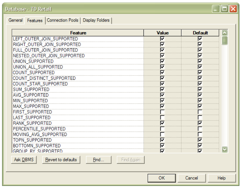
OBIEE Feature Table

When you import the schema or specify a database type in the General tab of the Database dialog box, the Feature table is automatically populated with default values appropriate for the database type.  The database dialog box can be found by selecting ‘properties’ after right clicking on the highest level folder in the physical model.

The feature table holds which SQL features the Analytics Server uses with this data source. You can tailor the default query features for a data source or database. For example, if “count distinct” operations don’t always perform well in your environment you can try turning this function off.  This may or may not help performance as OBIEE will pull back the list and do the count distinct on the server. 

Full outer joins are usually used by OBIEE when joining 2 fact tables via a dimension.   Depending upon the data this may or may not perform well.  Turning this feature off would force the server to do 1 query against each fact table and then join the results on the server.  If the result sets are small this could be faster than the full outer join. 
If you do choose to change the default settings just remember that this is the global default.  What helps one query may hinder another.

The drop down list for source database has 3 choices for Teradata.  The Teradata choice is actually mislabeled.  This actually has the settings for Teradata. There are no customizations required for the supported features settings.  If you do choose to change the default settings just remember that this is the global default.  Below is a screen shot of part of the Feature Table settings.

Connection Pool Configuration

The connection pool is an object in the Physical layer that describes access to the data source. It contains information about the connection between the Analytics Server and that data source.  The Physical layer in the Administration Tool contains at least one connection pool for each database. When you create the physical layer by importing a schema for a data source, the connection pool is created automatically. You can configure multiple connection pools for a database. Connection pools allow multiple concurrent data source requests (queries) to share a single database connection, reducing the overhead of connecting to a database.

Call Interface

During configuration of the connection pool you should ensure that the ‘call interface’ is set to the correct ODBC version.  This will maximize function shipping to the Teradata database.

Maximum Connections

For each connection pool, you must specify the maximum number of concurrent connections allowed. After this limit is reached, the Oracle BI Server routes all other connection requests to another allowed connection pool or, if no other allowed connection pools exist, the connection request waits until a connection becomes available.

Increasing the allowed number of concurrent connections can potentially increase the load on the underlying database accessed by the connection pool. Test and consult with
your DBA to make sure the data source can handle the number of connections specified in the connection pool. 

In addition to the potential load and costs associated with the database resources, the Oracle BI Server allocates shared memory for each connection upon server startup. This increases Oracle BI Server memory usage even if there is no activity.

When determining the number of concurrent connections you must not confuse users with connections.  For instance if you have on the average 10 users simultaneously hitting a dashboard that has 10 queries embedded then you have 10 users times 10 concurrent connections.  On the other hand if your users are only doing ad-hoc queries then you would only have 10 concurrent connections. 

Based on the number of concurrent queries, the Oracle Business Intelligence Server Administration Guide has the following advice for maximum connections:

“For deployments with Intelligence Dashboard pages, consider estimating this value at 10% to 20% of the number of simultaneous users multiplied by the number of requests on a dashboard. This number may be adjusted based on usage. The total number of all connections in the repository should be less than 800. To estimate the maximum connections needed for a connection pool dedicated to an initialization block, you might use the number of users concurrently logged on during initialization block execution.”

To restate a piece of Oracle’s advice – they believe that only 10-20% of simultaneous users are generating concurrent queries.  This obviously will vary by customer and should only be considered as a starting point for fine tuning.  The OBIEE online help states that you should have different connection pools for:

·      All Authentication and login-specific initialization blocks such as language, externalized strings, and group assignments.
·      All initialization blocks that set session variables.
·      All initialization blocks that set repository variables. These initialization blocks should always be run using the system Administrator user login.

Because each Oracle BI Server has an independent copy of each repository and hence its own back-end connection pools, back-end databases may experience as many as N*M connections, where N is the number of active servers in the cluster and M is the maximum sessions allowed in the connection pool of a single repository. Therefore, it may be appropriate to reduce the maximum number of sessions configured in session pools.

Other experts recommend:
·      Create a separate connection pool for the execution of aggregate persistence wizard. Remember that you need to give the schema user owner credentials for this connection pool as the wizard creates and drops tables
·      If need be create a separate connection pool for VIPs. You can control who gets to use the connection pool based on the connection pool permissions.

Lessons from Teradata Professionals
Advise from a Professional Services Consultant:

Concurrency is one of the trickiest questions to address in my experience. 500 concurrent users will likely not translate to 500 concurrent queries.

The OBIEE interface design will determine how many queries will be submitted concurrent with a single user accessing the page. If the queries are sub-optimal even a couple of them may cause issues.  When faced with such questions from the customer we have tried to highlight that it is query performance more than the concurrent users that will matter in the long run. If all the queries are well-tuned and finish in a few seconds, then it is not likely that one will see too many queries running concurrently on the system.

[At a large customer I] found that an OBIEE application having more than 500 users never had more than 10 users logged in simultaneously and even fewer queries running concurrently.

Advise from a Professional Services Consultant:

I had 8000 marketing and sales users on a system and they were targeting 50 concurrent users. In reality, we saw 12 max concurrent QUERIES with 1.5 to 2 being the normal load.

Use multiple BI users (connection pools) to access TD to spread the resources as we allocate spool, CPU, etc by user. Use the OBIEE cache facilities so as not to re-execute the queries for another user trying to get same info.

Define concurrency well before the test. Are they talking about 500 users logged on and doing normal work plus studying charts, getting coffee, etc, or 500 concurrent queries? They are vastly different…

Connection Pool Timeout

Connection pools work in conjunction with the “connection pooling timeout” setting.  The timeout specifies the amount of time, in minutes, that a connection to the data source will remain open after a request completes. During this time, new requests use this connection rather than opening a new one (up to the number specified for the maximum connections). The time is reset after each completed connection request.  If you set the timeout to 0, connection pooling is disabled; that is, each connection to the data source terminates immediately when the request completes. Any new connections either use another connection pool or open a new connection.

Multiple Connection Pools

The typical BI server will have one “connection pool” login to Teradata.  However, when different end-users need to be given different priorities on Teradata the single connection pool connection may not suffice.  In this case, multiple connection pools could be configured in the OBIEE physical layer.  Each connection pool user name can then be assigned a different Teradata account.  Multiple connection pools allow for multiple Teradata logins and therefore allow each login to each have its own priority/security assigned. 

Teradata Query Band Configuration

OBIEE can be set up for Teradata Query Banding (QB).  This should be considered a work-around until full query banding functionality is built into OBIEE.   To enable QB, the appropriate SQL is added as a connection script that is executed before each query.  This is found in the connection pool properties for the Teradata database.   On the “connection scripts” tab there is an “execute before query” section.  By clicking on the “new” button the following sql can be added:

set query_band = 'ApplicationName=OBIEE;ClientUser=valueof(NQ_SESSION.USER);' for session;

The metadata for the server needs to be reloaded via the Answers link or by restarting the OBIEE server.  The DBQL tables will then reflect the OBIEE user executing the query.   In this example the OBIEE server logs into TD with the user called sampledata.  Each OBIEE user is then identified with the query that they ran via the query band.  There are 2 users that ran OBIEE answer reports: demo and Administrator.

The query banding must be set for the session.  Setting for transaction won’t work due to the way that OBIEE sends the sql to Teradata.  Other arguments may be added to the query band.   

For more information on Query Banding in Teradata see the Teradata Orange Books “Using Query Banding in Teradata Database 12.0”, “Using Query Banding in
Teradata Database 13.0” and “Reserved QueryBand Names”.

Changing the Type of Source Database

If you have OBIEE configured against a warehouse and you forklift the warehouse to a different platform, Oracle fully supports changing the data source from the original platform to the new platform.  No other OBIEE configuration changes should be necessary.  If only forklifting a database was so easy!  No data type changes to worry about, no population scripts …
OBIEE has the capability to write data to the Teradata database.  This could be used by users who want to do planning or budgeting on a small scale. They could use OBIEE both as a reporting tool and also for entering sales quotas or budgets etc.  In Answers write-back is configured on a report by report basis.  The columns that are available for write-back appear in a box format for the end user.

There are multiple steps to configure write-back: 
  • The privilege must be explicitly granted to each user from Answers (even administrators).  The navigation path is: Answers > Settings > Administration > Manage Privileges > Write Back 
  • The column(s) that are to be written back to the database must then be identified in each Answers report.   Column Properties > Column Format tab > Value Interaction > Type > Write Back
  • Create a XML Template that holds the sql to execute for the write-back in the {ORACLEBI}/web/msgdb/customMessages folder.  You must include both an <insert> and an <update> element in the template. If you do not want to include SQL commands for one of the elements then you must insert a blank space between the unused opening and closing tags.
  • Set the write-back properties for the report.  The Write-back property button is only visible in Answers “table” view.

 Tips/Traps:
  • Each connection pool name must be unique in the entire .rpd file.
  • Make the table that write-back is enabled for “not cacheable”.  This is an attribute on the physical property box for the table under the “general” tab.